Class Activity (Week 11)

   This week node analysis, mesh analysis, and superposition analysis are use for circuits that contain 

resistors, inductors, and capacitors.

What is Vc in the below circuit?

Figure 1: Node Analysis and an Dependent-Current Source

Figure 2

Also source transformation is practiced again. 

 Thevenin and Norton equivalent circuits are a source transformation.

Figure 3: Thevenin and Norton equivalent circuits 

In order to find the Zth in a circuit, independent current sources must removed (open circuit), and 

independent voltage sources must short circuit. Then an arbitrary fixed current source or an arbitrary

fixed voltage source must connected to the points a and b.

Figure 4

Instantaneous and Average Power is discussed. 

  v(t) = V _m cos(ωt + θ _v )  ,  i(t) = I _m cos(ωt + θ _i )

Where V_m and I_m are the maximum values of v(t) and i(t), also θ_v and θ_i are the phase angles of the

voltage and current, respectively. The instantaneous power absorbed by the circuit is as below

formula.

p(t) = v(t)*i(t) , P(t) =  V _m I _m cos(ωt + θ _v ) cos(ωt + θ _i ) 

Pavg = ½ Re[VI*] = ½ V _m I _m cos(θ _v − θ _i )

According to average power, a resistor absorbs only power, while a inductor or a capacitor does not.

                                  
                                        MAXIMUM AVERAGE POWER TRANSFER


If Vth and Zth are used insted of a circuit, Maximum average power will occur under below 

conditions: 

Zth = Rth + j Xth     ,     Z_L = R _L + jX _L

Z_L = R _L + jX _L = R _Th − jX _Th = Z*_Th

The Maximum Average Power transferred is:        Pmax = |Vth|^2 / (8*Rth)   

Measuring Gain and Phase Difference

           A series circuit of two resistors are connected to a sinusoidal voltage, and its phase difference

between input and output is measured by a oscilloscope.

V(t) = Vm sin(ωt + Φ)  , Vm = 2v , Φ = 0°
 

Figure 1: Schematic of Series Circuit of two Resistors

Figure 2: Series Resistor Circuit with 1 KHz Frequency

f = 1/T , f = 1/(1 ms)  , f = 1 KHz

Figure 3: Series Resistor Circuit with 5 KHz Frequency

f = 1/ (200 μs) , f = 5 KHz

Figure 4: Series Resistor Circuit with 10 KHz Frequency

f = 1/T , f = 1/(100μs)  ,  f = 10 KHz

There are no phase difference between input and output in a pure resistive circuit.

Rtotal = R1 + R2 , Rtotal = 45.9 + 97.7 = 143.6 Ω

According to fig 2 and scale, 50 mA = 40 mm → I(total) = (10 mm)*(50 mA/40 mm) = 12.5 mA


Vout = R2*I(total)  , Vout(Measure) = (97.7Ω )*(12.5 mA) = 1.22 v 

G = Vout/Vin , G = 1.22/2 , G = 0.61

G(Theory) = Vout/Vin = R2/(R1+R2) , G(Theory) = 97.7/(97.7+45.9) = 0.68 

Gain Percent Error = [(0.68-0.61)/0.68]*100% = 10.3%

Figure 5: Series RL Circuit with an AC Voltage

Figure 6: Graph of Voltage and Current in an Series RL Circuit with 1 KHz Input Voltage

According to the Figure 6 and scale, Vout = (24 mm)*(200 mv/ 20 mm) = 240 mv (Blue graph)

VR1 = (35 mm)*(1v/ 20 mm) = 1.75 v , I(total) = (16 mm)*(50 mA/ 20 mm) = 40 mA

Inductor voltage (blue graph) leads current (small red graph) by 90 degree , and two red graph are in

phase because those show current and voltage of R1.

|XL| = (2π*1000)*(1mH) = 2π Ω , G(Measure) = Vout/Vin , G = 0.24/2 = 0.12 

G(Theory) = XL/Z , Z = 45.9 + j(2π) , G(Theory) = 0.136 ˂ 82.2°


Gain Percent Error = [(0.136 - 0.12)/0.136]*100% = 11.8%

Figure 7: Graph of Voltage and Current in an Series RL Circuit with 5 KHz Input Voltage

According to the Figure 7 and scale, Vout = (40 mm)*(500 mv/ 20 mm) = 1 v (Blue graph)

VR1 = (32 mm)*(1v/ 20 mm) = 1.6 v , I(total) = (14 mm)*(50 mA/ 20 mm) = 35 mA

Inductor voltage (blue graph) leads current (small red graph) by 90 degree , and two red graph are in

phase because those show current and voltage of R1.

 |XL| = (2π*5000)*(1mH) = 10π Ω  , G(Measure) = Vout/Vin , G = 1/2 = 0.5 

G(Theory) = XL / Z , Z = 45.9 +j(10π) , G(Theory) = 0.565 ˂ 55.6°

When frequency increases, XL, Vout, and G increases and vice versa.

Figure 8: A Practical Series RC Circuit

Figure 9: A Series RC Circuit

Figure 10: A Series RC Circuit with 1 KHz Frequency

According to the Figure 10 and scale, Vout = (29mm)*(1v/ 30 mm) = 0.97v (Blue graph)

 |XC| = 1/(2π*1000)*(0.41μF) = 388.4 Ω    ,   G(Measure) = Vout/Vin  , G = 0.97/2 = 0.485

 Z = 46.1 - j(388.4) , G(Theory) = XC / Z , G(Theory) = 0.993 ˂ -6.8°

Gain Percent Error = [(0.993 - 0.485)/0.993]*100% = 51.2%

Figure 11: A Series RC Circuit with 5 KHz Frequency

According to the Figure 11 and scale, Vout = (35 mm)*(1v/ 30 mm) = 1.17v (Blue graph)

 |XC| = 1/(2π*5000)*(0.41μF) = 77.68 Ω    ,   G(Measure) = Vout/Vin  , G = 1.17/2 = 0.585

G(Theory) = XC / Z , Z = 46.1 - j(77.68) , G(Theory) = 0.859 ˂ -30.7°

Gain Percent Error = [(0.859 - 0.585)/0.859]*100% = 31.9%

Figure 12: A Series RC Circuit with 10 KHz Frequency

According to the Figure 12 and scale, Vout = (45 mm)*(1v/ 40 mm) = 1.13 v (Blue graph)

 |XC| = 1/(2π*10000)*(0.41μF) = 38.9 Ω    ,   G(Measure) = Vout/Vin  , G = 1.13/2 = 0.565

G(Theory) = XC / Z , Z = 46.1 - j(38.9) , G(Theory) = 0.645 ˂ -49.9°

Gain Percent Error = [(0.645 - 0.565)/0.645]*100% = 12.4%

When frequency increases, XC, Vout, and G decreases and vice versa.

Class Activity (week #10)

This week concepts of phase difference, phasors, impedance, and admittance are taught.

Figure 1: Phase Difference between two waves

∆Φ = (2π) (∆t / T)

Figure 2: Schematic of Phase Difference of two Vectors

Figure 3: Relationship between Cartesian and Polar Coordinate Systems

Figure 4: Reciprocal Operation of two Voltage in Phasor Form

Figure 5: Time-Domain and Phasor-Domain Representation

Conversion of  V(t) = Vm sin(ωt + Φ) to V(t) = Vm cos (ωt + Φ - 90°) 

Figure 6: Conversion of a Voltage in Time Domain to Voltage in Phasor Domain

In phasor representation, just magnitude and phase difference of a voltage or current will represent.

Figure 7: Conversion of a Complex Number to Phasor Form

Figure 8: Conversion of Sum of Two voltage to Phasor Form

Rectangle form is easier when sum and subtraction of two or more voltage or current in time domain

are done. Phasor form is easier when multiplication and division of two or more voltage or current in

time domain are done. Phasor representation is useful when two voltages or currents have the same

frequency.

Figure 9: Impedance and Admittance

R = R     ,      XL = j(ωL)    ,    Xc = (1/ jωc) = -j / (ωc) 

Figure 10: Series Circuit Analysis with Phasors

Series RLC Circuit Step Response & RLC Circuit Response

       Series RLC Circuit Step Response

      The measured response of the series RLC second order circuit is compared with expectations

based on the damping ratio and natural frequency of the circuit.

 Vout(t) = Vc(t) = (1/C) ∫ i(t)*dt ,  Vin = Ri + VL + Vc , Vin(t) = Ri + L (di/dt) + Vc

R(di/dt) + L d[(di/dt)]/dt + dVc/dt = 0 , d²i/dt² + (R/L)* di/dt + (1/LC)*i = 0

i(t) = A*e^(St) , S^2 + (R/L)*S + /LC) = 0 ,  α = R/2L , ω_{0 = 1/ (LC)^(1/2)}

Figure 1: A series RLC Circuit

 A 2v square step input voltage is applied to the series RLC circuit. Oscilloscope channel one is

connected to the input of the circuit, and its second channel is also connected to the output.

Figure 2: A real Series RLC circuit

       This circuit is an under-damped because α ˂ ω_0. Resistance of resistor 0.9 Ω and capacitance 

of capacitor 4.26 μF are measured by a DMM. So damping factor α = 450000 (rad/s) , undamped 

natural frequency ω_{0 =} 484501.6 (rad/s) , ω_{d (Theory)} = 179560.0 (rad/s). 

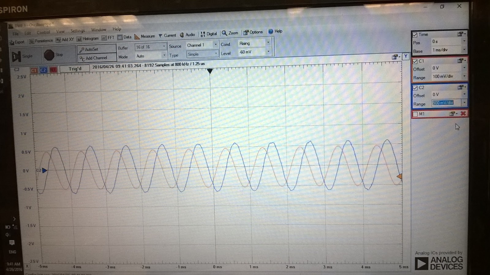
Figure 3: An Input-Output Graph of Series RLC circuit

According to the above graph, period of first under-damped output is 4 mm, also scale is 

1 ms = 100 mm. So (2π/ω_d ) = (4 mm)*(1 ms/100 mm) = 0.04 ms ,  ω_{d (Measure)} = 157000 (rad/s) ,

 f = 25000 Hz

Percent Error of damped natural frequency =  [(179560 - 157000)/(179560)]*100 = 12.6%

_{RLC Circuit Response}

       The measured response of a RLC second order circuit is compared with expectations

based on the damping ratio and natural frequency of the circuit. This circuit is an under-damped because α ˂ ω_0.

Figure 1: A RLC Second-Order Circuit

 A 2v square step input voltage is applied to the RLC circuit. Oscilloscope channel one is

connected to the output of the circuit, and its second channel is also connected to the input.

<sub>When input voltage is in its maximum (2v), capacitor will charge. When input voltage is equal zero, 

capacitor will parallel with L and R2. Of course, time constant of the capacitor is 

47*(8.13</sub> μF _{) = 382} μs , <sub>so the square input period should be equal or more than capacitor time

 constant. Internal resistance of inductor</sub> is measured 1.9 ohms by a DMM that is near to the R2.

  Ri + VL + Vc = 0 ,  Ri + L (di/dt) + Vc = 0

R(di/dt) + L d[(di/dt)]/dt + dVc/dt = 0 , d²i/dt² + (R/L)* di/dt + (1/LC)*i = 0


i(t) = A*e^(St) , S^2 + (R/L)*S + /LC) = 0 ,  α = R/2L , ω_{0 = 1/ (LC)^(1/2)}

ω_{0 =} [_{8.13E(-9)]^(-1/2) = 11090.6 (rad/s) ,}  ω_{d (Theory)} = 11076.95 (rad/s) , f = 1763.8 Hz 

Figure 2: A RLC Circuit with an Input Frequency equal 400 Hz

According to the above graph, period of the under-damped output is 40 mm, also scale is 

1ms = 60 mm. So (2π/ω_d ) = (40 mm)*(1 ms/60 mm) = (2/3) ms ω_{d (Measure)} = 9420 (rad/s) ,

 f = 1500 Hz. Vout(t) = R2*i(t).

Percent Error of damped natural frequency =  [(11076.95 - 9420)/(11076.95)]*100 = 14.96%

Figure 3: A Real RLC Circuit

Class Activity (Week 8)

     This week an integrator op-amp was ..... The output of an integrator op-amp is proportional to the

integral of its input signal.  Vout = (-1/RC) ∫Vin dt

Figure 1: An Integrator Op-amp Circuit

Figure 2: Input and Output Waveform of an Integrator Op-amp

The output of a differentiator op-amp circuit is proportional to the rate of change of its input signal.

Vout = - RC (dVin / dt)

Figure 3: An Differentiator Op-amp Circuit 

Figure 4: A Schematic of an Integrator and Differentiator Op-amp

Figure 5: Input and Output Wave Forms Of Op-amps

Figure 6: Input and Output of an Differetiator Op-amp

Also unit step, unit impulse, and unit ramp function is verified.

Figure 7: The Current of a Capacitor 

U(t) = 0 , t < 0. U(t) = 1 , t > 0. U(t) is undefined at t = 0.

The unit impulse function is derivative of the unit step function δ(t) .

δ(t) = 0 , t < 0 and t > 0. δ(t) is undefined at t = 0. 

R(t) = 0 , t < 0. R(t) = t, t ≥ 0.  

U(t) = dr(t) / dt , δ(t) = du(t) / dt

Figure 8: Response of a Capacitor Voltage and Capacitor Current to a Unit Step function

Inverting Differentiator

     The output of an inverting differentiator is derivative of its input. A sinusoidal input voltage is

connected to the op-amp with three different frequencies. Power supplies voltage of op-amp are ± 5v.

Figure 1: An Inverting Differentiator Op-amp

i) f = 1 KHz , amplitude = 200 mv , and offset = 0v

According to Volt/div of oscilloscope (measured voltage), Vin = 200 mv and Vout = 1000.25 mv

Vin = Asin(ωt) , Vout = Aω cos(ωt) , ω = 2πf  , Vout = -RC dVin / dt , Vout = -(RCAω)*cos(ωt)

If R = 1KΩ and C = 1μF so RC = 10E(-3). Vout = -(0.4π)*cos(ωt) , Vout = -1.257 *cos(ωt).

Output amplitude = -1257 mv.

percent error of output voltage = [(expected voltage - measured voltage) / expected voltage]*100%

percent error = [(1257 - 1000.25) / 1257]*100% = 22.43%

Figure 2: A Sinusoidal Input voltage of 1 KHz

ii) f = 2 KHz , amplitude = 200 mv , and offset = 0v

According to Volt/div of oscilloscope (measured voltage) , Vin = 200 mv and Vout = 2500 mv

Vin = Asin(ωt) , Vout = Aω cos(ωt) , ω = 2πf  , Vout = -RC dVin / dt , Vout = -(RCAω)*cos(ωt)

If R = 1KΩ and C = 1μF so RC = 10E(-3). Vout = -(0.8π)*cos(ωt) , Vout = -2.513 *cos(ωt).

Output amplitude = -2513 mv.

percent error of output voltage = [expected voltage - measured voltage| / expected voltage]*100%

percent error = [(2513 - 2500) / 2513]*100% = 0.52%

Figure 3: A Sinusoidal Input voltage of 2 KHz

iii) f = 500 Hz , amplitude = 200 mv , and offset = 0v

According to voltage div of oscilloscope (measured voltage), Vin = 200 mv and Vout = 500 mv

Vin = Asin(ωt) , Vout = Aω cos(ωt) , ω = 2πf  , Vout = -RC dVin / dt , Vout = -(RCAω)*cos(ωt)

If R = 1KΩ and C = 1μF so RC = 10E(-3). Vout = -(0.2π)*cos(ωt) , Vout = -0.6283 *cos(ωt).

Output amplitude = -628.3 mv.

percent error of output voltage = [expected voltage - measured voltage| / expected voltage]*100%

percent error = [(628.3 - 500) / 628.3]*100% = 20.42%

Figure 4: A Sinusoidal Input voltage of 500 Hz

According to the percent errors are calculated for three different frequencies, when f = 2 KHz percent

error is less than others low frequencies. In other words, percent error of output voltage decrease 

when frequencies increase.

Frequency (Hz)	Input Voltage (mv)	Expected Output Voltage (mv)	Measured Output Voltage (mv)	Percent Error%
500	200	500	628.3	20.42
1000	200	1257	1000.25	22.43
2000	200	2513	2500	0.52

Figure 5: A Schematic of an Inverting Differentiator Op-amp

When input voltage is 1 volt, the inverting differentiator op-amp will go to saturation state.

Vin = Asin(ωt) , Vout = Aω cos(ωt) , ω = 2πf  , Vout = -RC dVin / dt , Vout = -(RCAω)*cos(ωt)

If R = 1KΩ and C = 1μF so RC = 10E(-3). 

If f = 1 KHz. Vout = -(2π)*cos(ωt) , Vout = - 6.28 *cos(ωt).

Amplitude of output voltage is equal - 6.28 v  that is bigger than power supply voltage (± 5v).

Figure 6: An Inverting Differentiator Op-amp in Saturation Situation